The primary objective here is to make sure the framework I use in R to backtest strategies delivers similar results to that of MT4, most specifically to 99% tick accuracy MT4 backtesting. Why the 99% tick accuracy …. because it’s reproducible. A secondary outcome of this validation is to determine if backtesting could be carry on only in R, to benefit from enhanced statistical optimization, but in a time-efficient way when compared to MT4. Assuming positive outcomes, this will be followed by a post detailing the process of transferring a backtested strategy in R to production for MT4 demo-trading, prior live release.
MT4 Strategy used for validation: the SMA
I will investigate a Simple Moving Average (SMA) strategy, derived from this universalMACrossEA.mq4 MT4 script. The strategy is as follows: When FastMA (period=20) cross-up Slow MA (period=50), send a Buy and Close Sell, When FastMA cross-down SlowMA, Close Buy and Open Sell. EA Inputs are as follows (Refer to the figure below for a complete setup of strategy inputs): […] FastMAPeriod=20, FastMAType=0 […] SlowMAPeriod=50, SlowMAType=0 […] MinCrossDistance=0 […] StopAndReverse=false, PureSAR=true, ExitOnCross=true […] ; If I’m getting this thing right, it doesn’t matter what the other inputs are to obtain the desired behavior.
There follows the illustration of this SMA strategy backtested in MT4 with 99% tick accuracy, on GBPUSD Hourly (H1). Ah ! the 99% tick-by-tick backtesting in MT4, a whole story in itself but hopefully there are great tools out there to automate the process now. I personally use TickStory. The final drop to easily breath through that process is to download an old version of Metatrader that is compatible with TickStory ; I use an old Alpari NZ version 4.00 build 451 for that purpose w/o any account to prevent auto-updating. You may google mtjp4setup-451.exe to find proper builds. The complete MT4 Backtesting Strategy Report is available here.
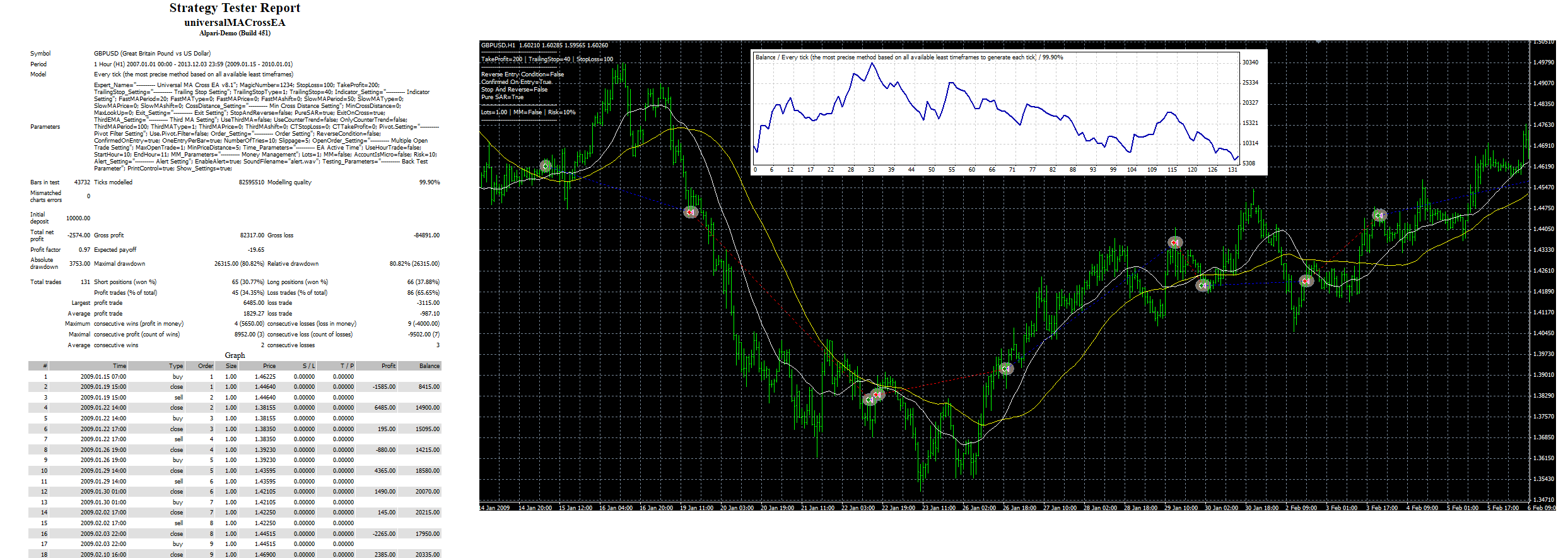
Strategy Tester Report with 99% tick-accuracy for SMA strategy
… discussing the interest of backtesting on tick-by-tick data for a strategy based on hourly stats is out of the present context – yet I do think this is not necessary but it looks good on the report !
R Backtesting Results on Equivalent SMA Strategy
Initial Test on hourly quotes not originating from the tick data
My first objective was to quickly determine whether or not there were supporting evidence that R & MT4 could provide the same results prior getting into precise testing. More specifically, as I’m interested in using the great framework designed by the Systematic Investor Toolbox for R (SIT), I’ve elected to reuse the Forex Intraday backtest example mixed with a later blog to implement the SMA strategy – The R-script is presented below (Thx to R syntax highlighting in wp.com) and you can see how simple it is , and thus how great the R SIT library is. It is worth noting that this design uses hourly historical Forex data from FXHISTORICALDATA.COM, that features hourly Low-High 4-digits quotes only, that are of no match to the 5-digits tick data quality provided by TickStory. Nonetheless, I felt this might give sufficient evidence, if lucky, to motivate further work.
con = gzcon(url('http://www.systematicportfolio.com/sit.gz', 'rb'))
source(con)
close(con)

#*****************************************************************
# Load historical data
#******************************************************************
load.packages('quantmod')

New_MA <- function (){
tickers = spl('GBPUSD')

capital = 10000

data <- new.env()
getSymbols.fxhistoricaldata(tickers, 'hour', data, download=TRUE)

#  bt.prep function merges and aligns all symbols in the data environment
bt.prep(data, align='remove.na', dates='2009::2010')

prices = data$prices
# n = len(tickers)
models = list()


#*****************************************************************
# Code Strategies
#******************************************************************
data$weight[] = NA
data$weight[] = 1
models$buy.hold = bt.run.share(data, clean.signal=TRUE
#,capital=capital
)

#*****************************************************************
# Code Strategies : SMA Fast/Slow cross over
#******************************************************************
sma.fast = SMA(prices, 20)
sma.slow = SMA(prices, 50)

# data$weight matrix holds weights (signals) to open/close positions.
data$weight[] = NA
data$weight[] = iif(cross.up(sma.fast, sma.slow), 1, iif(cross.dn(sma.fast, sma.slow), -1, NA))

# bt.run computes the equity curve of strategy specified by data$weight matrix
models$ma.cross = bt.run.share(data, clean.signal=TRUE, trade.summary = TRUE
, do.lag = 2
#, commission=0.0002
#, capital=capital
)

#*****************************************************************
# Code Strategies : MA Cross Over
#******************************************************************
#   sma = bt.apply(data, function(x) { SMA(Cl(x), 200) } )
#   data$weight[] = NA
#   data$weight[] = iif(prices >= sma, 1, 0)
#   sma.cross = bt.run(data, trade.summary=T)

#*****************************************************************
# Create Report
#******************************************************************

# plotbt.custom.report function creates the customized report, which can be fined tuned by the user
plotbt.custom.report(models$ma.cross, models$buy.hold)
plotbt.custom.report(models$ma.cross, models$buy.hold, trade.summary=TRUE)
strategy.performance.snapshoot(models, T)
models$ma.cross$trade.summary
}
Considering the modest quality of the Forex data used in R for that first test, a first step was to compare the Date & Time at which orders were past in both R and MT4 backtests. Thereafter are presented parts of the tables summarizing the results. Green marks indicate an Order Type & Time match, Orange marks indicate Order Type & Time (+/- 1Hour) match, and Red marks indicate Orders with time mismatches. The proportion of Green and Orange marks indicates a good correlation between the 2 backtests and support further investigation. I have briefly looked at the origin of the Red marks to found that, for example, MT4 data started on the Feb.22nd 2009, a Sunday, whereas the R data started on the 23rd at midnight. I had the feeling this was Broker-GMT related and didn’t feel like this should require further details.

Comparing Hourly backtested orders from R with MT4 tick-by-tick orders
… I couldn’t help myself but kept pushing my luck into investigating the magnitude of the Loss/Profits for each of R/MT4 orders, to quickly realize that the discrepancies between the two Forex data were to great for a more precise study. At this point we’ve been lucky enough and I need to load the 5-digits tick data into R for a comparable backtest and perform a thorough evaluation against the MT4 backtests.
Running a Backtest in R on Hourly Data derived from the Tick Data
In the SIT framework, the data variable returning the hourly-formatted tick data is as followed:
<br />> ls(data)<br />[1] "dates" "execution.price" "GBPUSD_hour" "prices" "symbolnames" "weight"<br />> ls.str(data)<br />dates : POSIXct[1:6171], format: "2009-01-11 21:00:00" "2009-01-11 22:00:00" "2009-01-11 23:00:00" "2009-01-12 00:00:00" "2009-01-12 01:00:00" ...<br />execution.price : An ‘xts’ object on 2009-01-11 21:00:00/2010-01-01 21:00:00 containing:<br />Data: num [1:6171, 1] NA NA NA NA NA NA NA NA NA NA ...<br />- attr(*, "dimnames")=List of 2<br />..$ : NULL<br />..$ : chr "GBPUSD_hour"<br />Indexed by objects of class: [POSIXct,POSIXt] TZ: GMT<br />xts Attributes:<br />NULL<br />GBPUSD_hour : An ‘xts’ object on 2009-01-11 21:00:00/2010-01-01 21:00:00 containing:<br />Data: num [1:6171, 1:4] 1.51 1.51 1.51 1.51 1.51 ...<br />- attr(*, "dimnames")=List of 2<br />..$ : NULL<br />..$ : chr [1:4] "Open" "High" "Low" "Close"<br />Indexed by objects of class: [POSIXlt,POSIXt] TZ: GMT<br />xts Attributes:<br />NULL<br />prices : An ‘xts’ object on 2009-01-11 21:00:00/2010-01-01 21:00:00 containing:<br />Data: num [1:6171, 1] 1.51 1.51 1.51 1.51 1.51 ...<br />- attr(*, "dimnames")=List of 2<br />..$ : NULL<br />..$ : chr "GBPUSD_hour"<br />Indexed by objects of class: [POSIXct,POSIXt] TZ: GMT<br />xts Attributes:<br />NULL<br />symbolnames : chr "GBPUSD_hour"<br />weight : An ‘xts’ object on 2009-01-11 21:00:00/2010-01-01 21:00:00 containing:<br />Data: num [1:6171, 1] NA NA NA NA NA NA NA NA NA NA ...<br />- attr(*, "dimnames")=List of 2<br />..$ : NULL<br />..$ : chr "GBPUSD_hour"<br />Indexed by objects of class: [POSIXct,POSIXt] TZ: GMT<br />xts Attributes:<br />NULL<br />
Now that I know the input format for SIT to work as-is, I move on to TickStory and look at the possible export format hoping I will not need to write an R-script to hourly-format the tick data myself. Luckily, I found that TickStory can output the following ‘Generic Bar Format’ = {BarBeginTime:yyyyMMdd},{BarBeginTime:HH:mm:ss},{Open},{High},{Low},{Close},{Volume} (told you it was a great piece of freeware); and that is the case for bar from 1 second to 1 week. Great ! The R function to read-in TickStory Generic Bar Format (hourly) into something SIT can digest, based on sourcing the SIT function getSymbols.fxhistoricaldata(…) is presented thereafter. For testing purposes, the output from TickStory for hourly bars from 2009.01.01 to 2010.01.01 is available here (396KB). One last thing I need to mention is that I have loaded information from my broker for TickStory to use a Spread of 20 on 5-digits, that is 2pips.
Note that this script is sensitive to the ‘Generic Bar Format’ – for now I’ll stick to what comes out of the box and we’ll see in the future how we’ll do things, specifically as you might have seen that the ‘Generic Tick Format’ differs from the ‘..Bar..’ one in that Dates and Times are 2 different columns for ‘..bar..’ and concatenated as a single column for ‘..tick..’ !
TickStory2SIT <- function (Symbols="GBPUSD", type="hour", env = .GlobalEnv,
                           file="Forex//TestData/GBPUSD_GenericBarFormat2009-2010.csv" , download = FALSE){

  # test file at https://drive.google.com/file/d/0BxMQxUqd263pTFFYV29IcmlHem8/edit?usp=sharing
  temp <- read.csv(file, sep = ",")
  out = xts(temp[3:6],
                 strptime(paste(temp$Date, temp$Timestamp), format='%Y%m%d %H:%M:%S'))
  assign(paste(gsub('\\^', '', Symbols), type, sep='_'), out, env)
  return(env)
}
Now, in the ‘New_MA <- function ()’ created previously replace the following lines to input the hourly tick-derived data we’ve just created:
  # tickers = spl('GBPUSD')
  capital = 10000
  data <- new.env()
  # getSymbols.fxhistoricaldata(tickers, 'hour', data, download=TRUE)
  TickStory2SIT("GBPUSD", "hour", data, file="./MT4ReportStatementAnalysis/TestData/GBPUSD_GenericBarFormat2009-2010.csv")
One final touch is to write a R function to load the MT4 Strategy Reports and further quantify potential differences between R and MT4 backtests :
MT4_ParseStrategyReport = function(SRname)
{
x = readHTMLTable(SRname)
#   > head(SR_Parsed)
#     1 2009.01.02 06:01   buy 1 0.02 1.38696 0.00000 1.38926            NA
#   2 2 2009-01-02 06:40   buy 2 0.04 1.38486 0.00000 1.38716          <NA>
#   3 3 2009-01-02 07:10   t/p 2 0.04 1.38716 0.00000 1.38716 9.20 10009.20
#   4 4 2009-01-02 07:10 close 1 0.02 1.38717 0.00000 1.38926 0.42 10009.62
perf <- NULL
perf$time <- as.character(x[[2]][,2])
perf$OrderType <- as.character(x[[2]][,3])
perf$OrderID <- as.double(as.character(x[[2]][,4]))
perf$LotSize <- as.double(as.character(x[[2]][,5]))
perf$Price <- as.double(as.character(x[[2]][,6]))
perf$SL <- as.double(as.character(x[[2]][,7]))
perf$TP <- as.double(as.character(x[[2]][,8]))
perf$Profit <- as.double(as.character(x[[2]][,9]))  ; perf$Profit[is.na(perf$Profit)] =0
perf$Balance <- as.double(as.character(x[[2]][,10])); perf$Balance[is.na(perf$Balance)] =0

table = getNodeSet(htmlParse(SRname),"//table") [[1]]
mypattern = '<td>([^<]*)</td>'
xt <- readHTMLTable(table,
header = c("Content"), colClasses = c("character"),
trim = TRUE, stringsAsFactors = FALSE
)
perf$Symbol <- unlist(strsplit(xt[[2]][1]," "))[[1]]

# desired structure
# symbol | weight | entry.date | exit.date | entry.price | exit.price | return
entry = which(!duplicated(perf$OrderID), arr.ind=TRUE)
ret <- NULL
for (i in 1:length(entry) ){
exit = which(perf$OrderID==perf$OrderID[entry[i]], arr.ind=TRUE)[2]
ret$symbol <- c( ret$symbol, perf$Symbol)

if (perf$OrderType[entry[i]]=="buy") {ret$weight <- c(ret$weight, perf$LotSize[entry[i]])}
else {ret$weight <- c(ret$weight, -perf$LotSize[entry[i]])}

ret$entry.date <- c(ret$entry.date, as.character(perf$time[entry[i]]) )
ret$exit.date <- c(ret$exit.date, as.character(perf$time[exit]) )
ret$entry.price <- c(ret$entry.price, perf$Price[entry[i]])
ret$exit.price <- c(ret$exit.price, perf$Price[exit])
ret$profit <- c(ret$profit, perf$Profit[exit])
} # VALIDATION: cumsum(ret$profit)+10000 #InitialDeposit=10000
return(ret)
}
NOTE: As I was validating this R function by comparing the cumulative returns obtained with R with that of MT4 Build 225 from the Strategy Test Report on INDRAFXSCALPING_V4.2, I realized that MT4 was off in calculating the ‘Balance=Equity at orders’ closes’ – refer to OrderID 45 to 49 ; kind of disappointing MT4 cannot even out put correct cumulative sums but I guess that’s what retail platform stands for (but hey, they do provide means to make $$ at a retail price – so I’m fine with it). Yet, I have to check if this was corrected in latter builds (we’ll see about that). Although I don’t have the same MT4 strategy to test, what i can say is that, with MT4 Build 451 from the Strategy Test Report on GBPUSD_2009_SMAcross (our real interest for that post), R cumulative sum of profits correlate with that of MT4.
Comparing the Results of Both Backtests on hourly data derived from tick data
Apple to Apple … that’s always the issue. Looking closely at the Hourly data derived from Tick data through TickStory I realized that Hourly {Open,Close,Low,High} are bid prices only (after comparing with the complete bid/ask quote on tick data). That’s the first thing to remember – THE SET-UP IS SUBOPTIMAL WHEN COMPARED TO LIVE TRADING CONSIDERING ONLY BID PRICES ARE USED (during live trading, you buy @ ask, and sell @ bid). However, looking at MT4 Strategy Report, I could not explain the execution prices from the tick data (weird right!). Anyways, I’ll come to this later – here is a quick analysis of the SIT Vs MT4.
First you will need to re-source this function to update the SIT trade.summary function and enable 5-digits precision in the report (instead of the rounding 2-digits).
bt.trade.summary <- function
(
  b,
  bt, Rounding=5
)
{

  if( bt$type == 'weight') weight = bt$weight else weight = bt$share
  out = NULL
  weight1 = mlag(weight, -1)
  tstart = weight != weight1 & weight1 != 0
  tend = weight != 0 & weight != weight1
  tstart[1, weight[1,] != 0] = T
  trade = ifna(tstart | tend, FALSE)
  prices = b$prices[bt$dates.index,,drop=F]
  if( sum(trade) > 0 ) {
    execution.price = coredata(b$execution.price[bt$dates.index,,drop=F])
    prices1 = coredata(b$prices[bt$dates.index,,drop=F])
    prices1[trade] = iif( is.na(execution.price[trade]), prices1[trade], execution.price[trade] )
    prices1[is.na(prices1)] = ifna(mlag(prices1), NA)[is.na(prices1)]
    prices[] = prices1
    weight = bt$weight
    symbolnames = b$symbolnames
    nsymbols = len(symbolnames)
    trades = c()
    for( i in 1:nsymbols ) {
      tstarti = which(tstart[,i])
      tendi = which(tend[,i])
      if( len(tstarti) > 0 ) {
        if( len(tendi) < len(tstarti) ) tendi = c(tendi, nrow(weight))
        trades = rbind(trades,
                       cbind(i, weight[(tstarti+1), i],
                             tstarti, tendi,
                             as.vector(prices[tstarti, i]), as.vector(prices[tendi,i])
                       )
        )
      }
    }
    colnames(trades) = spl('symbol,weight,entry.date,exit.date,entry.price,exit.price')
    out = list()
    out$stats = cbind(
      bt.trade.summary.helper(trades),
      bt.trade.summary.helper(trades[trades[, 'weight'] >= 0, ]),
      bt.trade.summary.helper(trades[trades[, 'weight'] <0, ])
    )
    colnames(out$stats) = spl('All,Long,Short')
    temp.x = index.xts(weight)
    trades = data.frame(coredata(trades))
    trades$symbol = symbolnames[trades$symbol]
    trades$entry.date = temp.x[trades$entry.date]
    trades$exit.date = temp.x[trades$exit.date]
    trades$return = round(100*(trades$weight) * (trades$exit.price/trades$entry.price - 1),Rounding)
    trades$entry.price = round(trades$entry.price, Rounding)
    trades$exit.price = round(trades$exit.price, Rounding)
    trades$weight = round(100*(trades$weight),Rounding)
    out$trades = as.matrix(trades)
  }
  return(out)
}
The you may use this to quickly compare Priece Entry differences and Profits Differences:
###########################
# Entry Price Comparison
##########################
SIT <- as.data.frame(models$ma.cross$trade.summary[2])
l = length(ret$entry.date)

DiffInSeconds = abs(as.POSIXct(strptime(ret$entry.date[2:l], "%Y.%m.%d %H:%M")) -
as.POSIXct(strptime(SIT$trades.entry.date, "%Y-%m-%d %H:%M")) )

SIT$trades.entry.date[which(DiffInSeconds>0)]
ret$entry.date[which(DiffInSeconds>0)+1]

############################
# Entry Price Comparison
############################
DiffInEntryPrice = abs(as.double(paste(ret$entry.price[2:l])) - as.double(paste(SIT$trades.entry.price)))

###############################
# Profits Comparison
##############################

MT4Prof = (as.double(paste(ret$entry.price[2:l])) - as.double(paste(ret$exit.price[2:l]))) * (-ret$weight[2:l])
RProf = (as.double(paste(SIT$trades.entry.price)) - as.double(paste(SIT$trades.exit.price))) * (-as.double(paste(SIT$trades.weight))/100)

formatC(100*abs(MT4Prof - RProf) / abs(MT4Prof), format="fg")

###########################
# Order Type Comparison
###########################
max(cumsum(ret$weight[2:l] - as.double(paste(SIT$trades.weight))/100))
The results will be as follows:
<br /><br />> ###########################<br />> # Entry Price Comparison<br />> ##########################<br />> SIT l = length(ret$entry.date)<br />><br />> DiffInSeconds = abs(as.POSIXct(strptime(ret$entry.date[2:l], "%Y.%m.%d %H:%M")) -<br />+ as.POSIXct(strptime(SIT$trades.entry.date, "%Y-%m-%d %H:%M")) )<br />> DiffInSeconds<br />Time differences in secs<br /> [1] 0 0 0 0 0 0 0 0 0 0 0 0 0 0 0 0 0 0 0 0 0 3600 0 0 0 0 0<br /> [28] 0 0 0 0 0 0 0 0 0 0 0 0 0 0 0 0 0 0 0 0 3600 0 0 0 0 0 0<br /> [55] 0 0 0 60 0 0 0 0 0 0 0 0 0 0 0 0 0 0 0 0 0 0 0 0 0 0 0<br /> [82] 0 0 0 0 3600 0 0 0 0 0 3600 0 0 0 0 0 0 3600 3600 0 0 0 0 0 0 3600 0<br />[109] 0 0 0 0 0 0 0 0 3600 3600 0 3600 0 0 0 0 0 0 0 0 0 0 0<br />attr(,"tzone")<br />[1] "GMT"<br /><br />> DiffInEntryPrice = abs(as.double(paste(ret$entry.price[2:l])) - as.double(paste(SIT$trades.entry.price)))<br />> DiffInEntryPrice<br /> [1] 0.00110 0.00590 0.00685 0.00335 0.00155 0.00790 0.00240 0.00295 0.00240 0.00905 0.00150 0.00020 0.00025 0.00180 0.00135 0.00290<br /> [17] 0.00156 0.00805 0.00815 0.00150 0.00120 0.00075 0.00115 0.00095 0.00460 0.00195 0.00415 0.00210 0.00550 0.00185 0.00275 0.00065<br /> [33] 0.00085 0.00265 0.00170 0.00075 0.00005 0.00280 0.00225 0.00090 0.00012 0.00065 0.00210 0.00065 0.00047 0.00030 0.00200 0.00295<br /> [49] 0.00000 0.00455 0.00225 0.00218 0.00500 0.00007 0.00203 0.00370 0.00078 0.00010 0.00015 0.00545 0.00055 0.00425 0.00175 0.00175<br /> [65] 0.00140 0.00210 0.00140 0.00095 0.00060 0.00170 0.00055 0.00460 0.00010 0.00000 0.00185 0.00140 0.00145 0.00005 0.00250 0.00180<br /> [81] 0.00215 0.00320 0.00075 0.00030 0.00000 0.00215 0.00240 0.00185 0.00320 0.00000 0.00060 0.00405 0.00200 0.00080 0.00030 0.00360<br /> [97] 0.00105 0.00150 0.00710 0.00015 0.00105 0.00260 0.00090 0.00485 0.00010 0.00520 0.00475 0.00370 0.00310 0.00235 0.00200 0.00130<br />[113] 0.00150 0.00085 0.00420 0.00005 0.00355 0.00085 0.00050 0.00010 0.00160 0.00120 0.00075 0.00046 0.00085 0.00135 0.00055 0.00126<br />[129] 0.00015 0.00015 0.00015<br /><br />> formatC(100*abs(MT4Prof - RProf) / abs(MT4Prof), format="fg")<br /> [1] "30.28" "19.66" "523.1" "20.45" "21.65" "69.13"<br /> [7] "37.93" "23.62" "27.88" "47.63" "5.457" "3.448"<br /> [13] "18.9" "4.39" "48.44" "14.66" "307.6" "102.2"<br /> [19] "140" "5.825" "26.47" "7.143" "1.19" "21.6"<br /> [25] "10.25" "10.86" "5.647" "73.91" "73.87" "20"<br /> [31] "9.722" "6.148" "10.91" "4.308" "5.864" "6.829"<br /> [37] "18.46" "54.01" "25.1" "3.982" "6.476" "16.13"<br /> [43] "11.51" "2.287" "2.081" "9.524" "10.8" "16.76"<br /> [49] "107.1" "10.98" "23.75" "23.81" "12.11" "155.6"<br /> [55] "46.59" "57.94" "30.77" "2.024" "35.45" "36.04"<br /> [61] "800" "23.12" "0" "53.39" "102.9" "3.271"<br /> [67] "51.09" "16.28" "34.85" "26.32" "55.38" "54.65"<br /> [73] "0.3552" "7.66" "60.75" "95" "466.7" "51"<br /> [79] "8.046" "7.865" "35" "158.1" "5.202" "2.344"<br /> [85] "37.07" "40.81" "2.813" "36.33" "47.76" "2.797"<br /> [91] "202.2" "96.03" "7.818" "37.93" "29.07" "17.85"<br /> [97] "318.8" "162.3" "64.95" "8.491" "13.78" "55.74"<br />[103] "12.92" "89.62" "196.3" "265.3" "20.39" "30.77"<br />[109] "2.693" "12.07" "36.07" "16.87" "29.55" "54.47"<br />[115] "27.85" "47.37" "31.88" "6.995" "6.63" "6.883"<br />[121] "37.33" "5.028" "6.971" "3.858" "9.462" "6.4"<br />[127] "20.94" "178.5" "0" "0.000000000001283" "1.641"<br />> max(cumsum(ret$weight[2:l] - as.double(paste(SIT$trades.weight))/100))<br />[1] 0<br />> ###########################<br />> # Order Type Comparison<br />> ###########################<br />> max(cumsum(ret$weight[2:l] - as.double(paste(SIT$trades.weight))/100))<br />[1] 0<br /><br />
Conclusion
- MT4 execution prices could not be explained from the Tick Data, even when accounting for the fixed spread (2pips), although such execution price is close to Bar-Open (+/- spread).
- SIT uses Bar-Close as the execution price for both Entry Price and Exit Price.
- MT4 and SIT Profits do not match in this testing due to (1) and (2).
- MT4 and R Order Sequence does match perfectly
- MT4 and R Entry Time are really close, at most separate by a Bar (a hour in our case).
- Based on (4) and (5) I would suggest that R “has the potential” to serve as an accurate backtesting framework, although SIT and Quantmod, used as-is, are not optimal.
- THE QUALITY OF THIS BACKTESTING SET-UP IS SUB-OPTIMAL – our primary objective was off as it assumed MT4 99% tick data backtesting was accurate, but no evidence of such assumption was found.
Running a Backtest in R on Raw Tick Data
As you may think, I was really not happy with this situation. So I decided not to leverage a high-level R framework such as SIT, but to directly get to R’s Quantmod framework.
I wrote a simple R function to load tick data into R xts objects. For that purpose I have created with TickStory a one day tick data file with the following format: {Timestamp:yyyyMMdd} {Timestamp:HH:mm:ss:fff},{BidPrice},{AskPrice},{BidVolume},{AskVolume}
loadDukaTick <- function(file = "Forex//TestData/GBPUSD_GenericTickCommaDelimited.csv") {
  tick <- read.csv(file, sep = ",")

  # TEST DATA: https://drive.google.com/file/d/0BxMQxUqd263pTXpTb1plN1AtTm8/edit?usp=sharing

  # Tick Data Format - verify with TickStory when exporting
  # Timestamp Bid.price Ask.price Bid.volume Ask.volume
  # 1 20090111 21:00:17:245   1.51295   1.51345        4.2        1.2

  # set options to format the R Session with milliseconds - https://stat.ethz.ch/pipermail/r-help/2007-June/134006.html
  options("digits.secs"=6)
  # Sys.time()

  # Answer 2: http://stackoverflow.com/questions/13613655/colon-in-date-format-between-seconds-and-milliseconds-how-to-parse-in-r
  # To emphasize that a bit, %OS represents the seconds including fractional seconds ---
  # not just the fractional part of the seconds: if the seconds value is 44.234, %OS or %OS3 represents 44.234, not .234
  # So the solution is indeed to substitute a . for that final :
  ## gsub(":", ".", tick[,1])

  # Create zoo objects and append in series - http://shemz.wordpress.com/2013/02/15/download-fx-tick-data-using-r/
  # tick[, 2:3] <-> Bid and Ask, discarding the Volume
  # heavily inspired from http://shemz.wordpress.com/2013/02/15/download-fx-tick-data-using-r/
  dates <- as.POSIXct(strptime(gsub(":", ".", tick[,1]), "%Y%m%d %H.%M.%OS"))

  TickData <- zoo(tick[, 2:3], dates)
  tick <- NULL
  tick$bid = as.xts(TickData[, colnames(TickData) != "Bid.price"])
  tick$ask = as.xts(TickData[, colnames(TickData) != "Ask.price"])

  return (tick)
}
Then I wrote a very simple Quantmod backtest on these.
BasicQuantmodBacktest <- function (price){
  load.packages('quantmod')
  # http://blog.fosstrading.com/2011/03/how-to-backtest-strategy-in-r.html
  ## dvi <- DVI(price)
  sma.fast = SMA(price, 20)
  sma.slow = SMA(price, 50)

  # create signal: (long (short) if DVI is below (above) 0.5)
  # lag so yesterday's signal is applied to today's returns
  ## sig <- Lag(ifelse(dvi$DVI < 0.5, 1, -1))
  sig <- Lag(iif(cross.up(sma.fast, sma.slow), 1, iif(cross.dn(sma.fast, sma.slow), -1, NA)))

  FirstOrder <- which(!is.na(sig))[1]
  # Order <- which(!is.na(sig))

  for (i in 1:(FirstOrder-1) ){
    if (is.na(sig[i])) sig[i] <- -sig[FirstOrder]
  }

  for (i in (FirstOrder+1):length(sig)){
    if (is.na(sig[i])) sig[i] <- sig[i-1]
  }

  # calculate signal-based returns
  ret <- ROC(price)*sig #roc <- x/lag(x, n, na.pad = na.pad) - 1
  # FOR TESTING: subset returns to match data in Excel file
  # ret <- ret['2009-01-11/2009-01-11']
  eq <- exp(cumsum(na.exclude(ret)))
  plot(eq)

  # use the PerformanceAnalytics package
  # install.packages("PerformanceAnalytics")
  require(PerformanceAnalytics)
  # create table showing drawdown statistics
  table.Drawdowns(ret, top=10)
  # create table of downside risk estimates
  # table.DownsideRisk(ret)
  # chart equity curve, daily performance, and drawdowns
  charts.PerformanceSummary(ret)
}
Finally, those scripts run with
data = loadDukaTick();
BasicQuantmodBacktest(data$ask)
#####
# OR
#####
data=new.env();
TickStory2SIT("GBPUSD", "hour", data, file="./MT4ReportStatementAnalysis/TestData/GBPUSD_GenericBarFormat2009-2010.csv")
bt.prep(data, align='remove.na', dates='2009::2010')
prices = data$prices
BasicQuantmodBacktest(prices);
 which we compare to this in MT4
That’s it for today. Definitely not perfect, but as I’ve learnt through research, sometimes it’s good to publish something that did not work properly for the community to learn from undesirable methodologies, inefficient testing and, in our case, improper tools used for testing. From there, I will spend a little more time on defining the optimal behavior of a backtest engine with these tick data and such simple strategy. In truth, I’ve already looked at different python framework as my little finger’s telling me that R+python might be a good option.
HTH – keep me posted on your thoughts folks.
PS: As I was looking for importing the Dukascopy data into R, I’ve stumbled upon a R-parser for Gain Capital Forex data – If time is on my side, I’ll have a look as well.

You’ll need to download the MQL code snippet to enable your EA to be properly backtested using tick data & price based charts.
Is this what you are talking about regarding the MQL code snippet?
#include
and at the very top of the void OnTick() function add the following function call:
if(skipFirstTickOnBacktest()) return;
Maybe XmPh can help use validate this.
Thanks for an interesting post. What’s the logic in filling the gaps?
FirstOrder <- which(!is.na(sig))[1]
# Order <- which(!is.na(sig))
for (i in 1:(FirstOrder-1) ){
if (is.na(sig[i])) sig[i] <- -sig[FirstOrder]
}
for (i in (FirstOrder+1):length(sig)){
if (is.na(sig[i])) sig[i] <- sig[i-1]
}
Why not replace NAs with zeroes, not previous trading signals?
Nice analysis — thank you for posting this. In the first code box (Initial Test on hourly quotes not originating from the tick data), line 10 looks garbled. Would you please re-post that code?
Hi David, you were definitely right. I’ve re-posted the complete source code as elements were missing here and there. I’ve problems with “keeping the format right in R for presentation within wordpress” so I realized that outputs have been scrambled with HTML code in the process. Eventually, I’ll clean that up but at least the code is fine now (I’ve re-tested it all).